A Minimal Env

In this tutorial we’re going to write the simplest possible environment. We’re going to make something that has an agent moving around and getting visual observations of the world around it. We’re going to be able to record animations of that agent’s exploration, and we’re going to generate a neural net that can control it.

It might not look like much, but this is the basis off which we’ll later build an exploration env and an deathmatch env. Getting this boring little environment working first will let us discuss a lot of the fundamentals of megastep without getting caught up in the details of a specific task.

This is a very detailed tutorial. It’s 2,500 words to discuss fifty lines of code. If you’d prefer to explore the libary on your own, take a look at Playing With Megastep.

Setup

It’d a good idea to open yourself a Jupyter notebook or colab and copy-paste the code as you go, experimenting with anything you don’t quite understand.

In a pinch, you can also try things out in this Google Colab. The main problem is the font rendering is a bit weird.

Once you’ve got your notebook up and running, the first thing to do is to install megastep, and the extra demo dependencies, which should be as simple as running

!pip install git+https://github.com/andyljones/megastep[cubicasa,rebar] --yes

in a cell.

Geometry

The place to start is with the geometry. The geometry describes the walls, rooms and lights of an environment. In later tutorials we’re going to generate thousands of unique geometries, but here for our simplest-possible env, a single geometry will do. A single, simple geometry:

from megastep import geometry, toys

g = toys.box()
geometry.display(g)

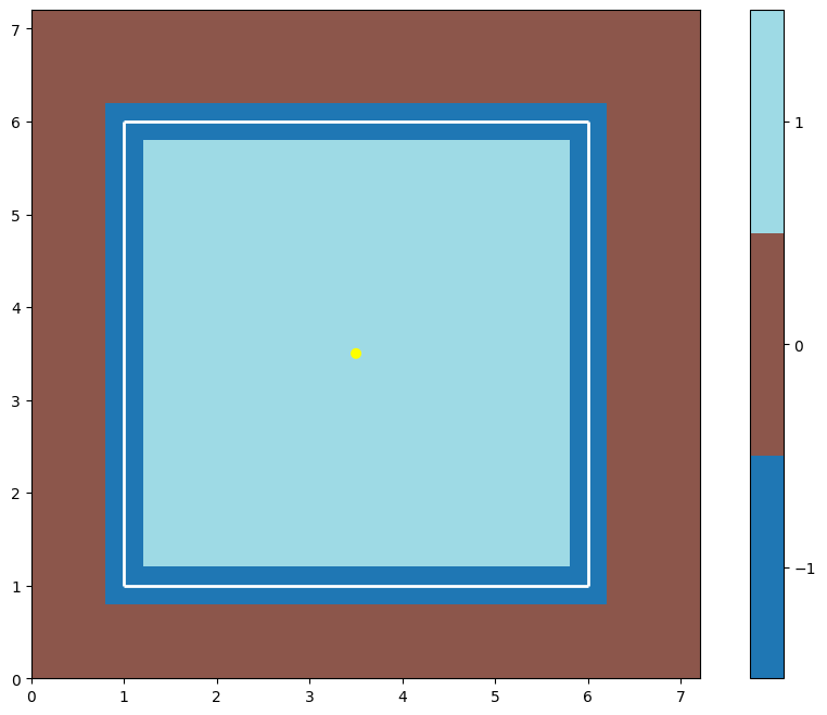
Yup, it’s a box. Four walls and one room. There’s more below about how the geometry is made, and also a brief discussion of its place in megastep.

Scenery

A geometry on its own is not enough for the renderer to go on though. For one it’s missing texture, and for two it only describes a single environment, when megastep’s key advantage is the simulation of thousands of environments in parallel. To turn the geometry into something the renderer can use, we turn it into a Scenery:

from megastep import scene
geometries = 128*[toys.box()]
scenery = scene.scenery(geometries, n_agents=1)

scene.display(scenery, e=126)

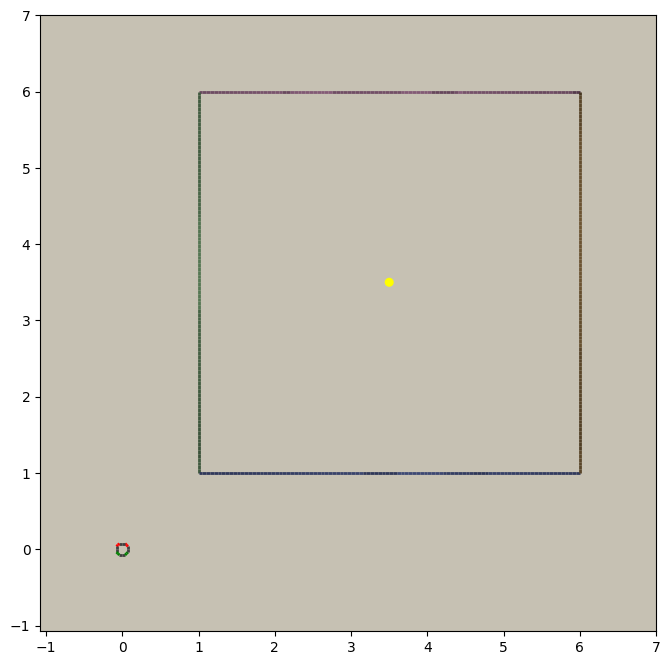
This code creates scenery for 128 copies of our box geometry, each with a randomly-chosen colourscheme and texture. One copy - copy #126 - is shown. You’ll also notice a model of an agent has also been created and placed at the origin. If you want to know more about what’s going on here, there’s another brief discussion about scenery and a tutorial on writing your own scenery generator.

Rendering

With the scenery in hand, the next thing to do is create a Core:

from megastep import core
c = core.Core(scenery)

The Core doesn’t actually do very much; there’re little code in it and all its variables are public. It does do some setup for you, but after that it’s just a bag of useful attributes that you’re going to pass to the physics and rendering engines.

One of things the core sets up is the Agents datastructure, which stores where the agents are. You can take a look with

>>> import torch
>>> c.agents.positions
tensor([[[0., 0.]],
        ...
        [[0., 0.]]], device='cuda:0')

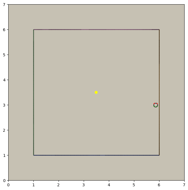
but all it’s going to tell you is that they’re at the origin. megastep stores all its state in PyTorch tensors like these, and it’s a-okay to update them on the fly. By default the origin is outside the box we’ve built, so as a first step let’s put them inside the box

c.agents.positions[:] = torch.as_tensor([3., 3.], device=c.device)

And now we can render the agents’ view

from megastep import cuda
r = cuda.render(c.scenery, c.agents)

This r is a Render object, which contains a lot of useful information that you can exploit when desiging environments. Principally, it contains what the agents see

from megastep import plotting
im = (r.screen
        [[0]]            # get the screen for agents in env #0
        .cpu().numpy())  # move them to cpu & numpy
plotting.plot_images({'rgb': im}, transpose=True, aspect=.1)

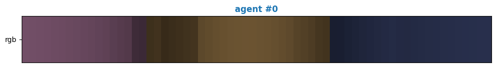
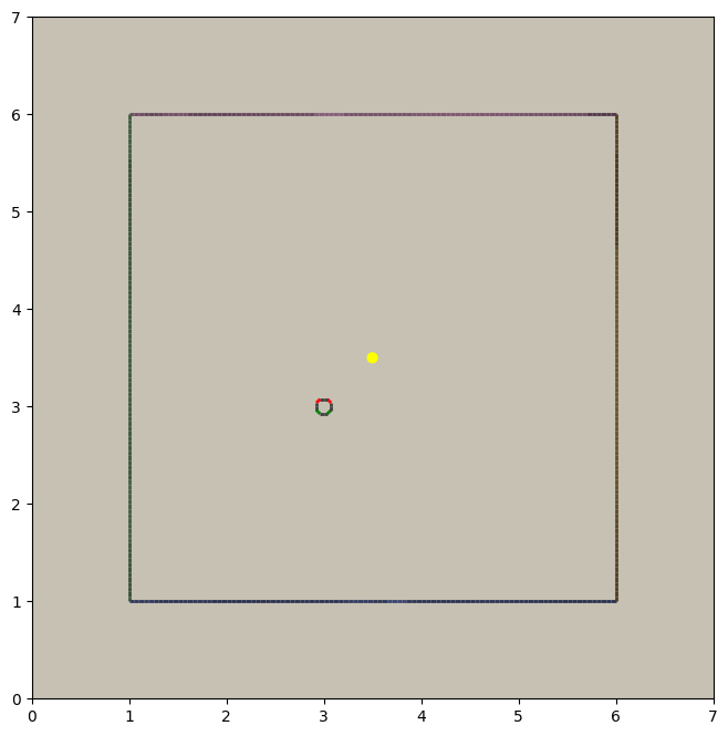
This is a 1-pixel-high image out from the front of the agent. You can read more about the rendering system in this section. As well as filling up the Render object, calling render does something else: it updates the agents’ models to match their positions. Having moved all the agents to (3, 3) earlier by assigning to c.agents.positions, plotting the scenery again shows that the agents’ models have moved from the origin to (3, 3):

scene.display(scenery)

Physics

Along with render(), the other important call in megastep is physics(). This call handles moving agents based on their velocities, and deals with any collisions that happen. If we set the agents’ velocities to some obscene value, then make the physics call:

>>> c.agents.velocity[:] = torch.as_tensor([1000., 0.], device=c.device)
>>> p = cuda.physics(c.scenery, c.agents)
>>> c.agents.positions
tensor([[[5.8649, 3.0000]],
        ...
        [[5.8649, 3.0000]]], device='cuda:0')

we see that afterwards, the agents positions have been updated to where the right wall is. If we check the scenery right now though, the agents’ models will still be at (3, 3) however. To update them, we need to call render again:

cuda.render(c.scenery, c.agents)
scene.display(c.scenery)

A Skeleton

We’ve now illustrated the basic loop in megastep:

g = toys.box()
scenery = scene.scenery(n_envs*[g], n_agents=1)
c = cuda.Core(scenery)

# set agent location
r = cuda.render(c.scenery, c.agents)
# generate an observation and send it to the agent
while True:
    # process decisions from the agent
    p = cuda.physics(c.scenery, c.agents)
    # post-collision alterations
    r = cuda.render(c.scenery, c.agents)
    # generate an observation and send it to the agent

This loop will be hiding at the bottom of any environment you write. For the purposes of actually using the environment though, that ‘while’ loop needs to be abstracted away. The typical way to do this follows from the OpenAI Gym, and while we’re not going to follow their interface exactly we are going to steal the ideas of a ‘reset’ method and a ‘step’ method:

class Minimal:

    def __init__(self, n_envs):
        geometries = n_envs*[toys.box()]
        scenery = scene.scenery(geometries, n_agents=1)
        self.c = cuda.Core(scenery)

    def reset(self):
        # set agent location
        r = cuda.render(self.c.scenery, self.c.agents)
        # generate an observation and send it to the agent
        return world

    def step(self, decision):
        # process decisions from the agent
        p = cuda.physics(self.c.scenery, self.c.agents)
        # post-collision alterations
        r = cuda.render(self.c.scenery, self.c.agents)
        # generate an observation and send it to the agent
        return world

This is exactly the same code as was in the loop, just with the interation with the agent made explicit through ‘decision’ and ‘world’ variables. This is very my syntactic sugar for agent-env interactions, and while I think it works well, you’re free to replace with your own. With this sugar though, the loop becomes much more flexible:

env = Minimal()
world = env.reset()
while True:
    decision = agent(world)
    world = env.step(decision)

Now all that’s left to be done is to fill out those comment lines.

An Aside

Now that we’re building up a class, it’s going to be impractical for me to copy-paste the source every time I discuss a change. Instead, you should grab the completed Minimal class from megastep’s demo module:

from megastep.demo.envs.minimal import *
self = Minimal()
world = self.reset()

The remainder of the code segments will be small ‘experiments’ - for want of a better word - you can run on this env to understand what’s happening and why it’s set up the way it is. If you want to play with the class’s definition, then open an editor at self.__file__ and copy-paste the contents into your notebook.

(You could alternatively edit it in-place, or copy it into a file ofyour own. Both of those however either require restarting the kernel after each edit, or setting autoreload up. Autoreload is magical and absolutely worth your time, but it is a tangent from this tutorial)

Spawning

Back to those comment lines! It’s a good idea to work through them in order, since that means you can validate that things are working as expected as you go. The first comment line is to ‘set agent location’. We’re going to want to do this on the first reset, and then every time the agent collides with something and needs to be respawned at a new location.

This is a pretty common task when building an environment, and so there’s a RandomSpawns module to do it for you. It gets added to the env in __init__,

from megastep import modules
self.spawner = modules.RandomSpawns(geometries, self.core)

and then you can call it with a mask of the agents you’d like to be respawned:

reset = self.core.agent_full(True)
self.spawner(reset)

As an aside, the agent_full() and env_full() methods will create on-device tensors for you of shape (n_env, n

This will move each agent to a random position in the room. You can see this directly by inspecting self.core.agents.positions, or you can render and display it:

self.core.render(self.core.scenery, self.core.agents)
scene.display(self.core.scenery)

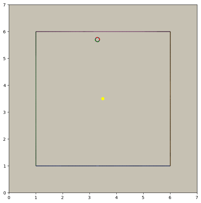
You can read more about how the respawning module works in the RandomSpawns documentation.

Observations

The next comment is ‘generate an observation and send it to the agent’. For our minimal environment, the observation will be a ye olde fashioned RGB (red-green-blue) camera, and again there’s a module for that:

self.rgb = modules.RGB(self.core)

This time, calling it gives you back a (n_env, n_agent, 3, 1, res)-tensor, suitable for passing to a PyTorch convnet:

obs = self.rgb()

The render method is called internally by rgb, saving us from having to do it explicitly ourselves. The class documentation for RGB has more details on how it works.

Following the decision-and-world setup, this obs gets wrapped in a arrdict so that if we decide to nail any other information onto the side of our observations, it’s easy to do so. That means our reset method in all its glory is

def reset(self):
    self.spawner(self.core.agent_full(True))
    return arrdict.arrdict(obs=self.rgb())

>>> self.reset()
arrdict:
obs    Tensor((128, 1, 1, 1, 64), torch.float32)

Actions

The third comment is ‘process decisions from the agent’. In our environment the action is simply whether to move forward/backward, left/right, or turn left/right. Once again, there’s a module for this:

self.movement = modules.SimpleMovement(self.core)

In the decision-and-world setup, the agent produces a decision arrdict with an "actions" key. The SimpleMovement module expects the actions to be an integer tensor, with values between 0 and 7. Each integer corresponds to a different movement. We can mock a decisions dict easily enough:

decision = arrdict.arrdict(actions=self.core.agent_full(3))

and calling the movement module will shift the agents forward:

self.movement(decision)

As with the depth module, the movement module makes the physics call internally, again saving us from having to do it ourselves. Like before, the class documentation for SimpleMovement has more details on how it’s implemented.

Having implemented both actions and observations, we can now assemble our step method:

def step(self, decision):
    self.movement(decision)
    return arrdict(obs=self.rgb())

Agent

That’s it. That’s the functional part of the environment done. All that’s left is to wire up an agent to it, and then watch it run.

When you’re doing reinforcement learning research, it helps if when you change the observations your environment emits, or the action spaces your environment takes, the network you’re using to run your agent adapts automatically. The megastep way to do this is to set .obs_space and .action_space on your environment, and then use a library of heads to automatically pick the inputs and outputs of your network.

Using heads to create a network looks like this:

intake = heads.intake(env.obs_space, width)
output = heads.output(env.action_space, width)

You ask for an intake that conforms to the observation space, and outputs a vector of a specified width. Similarly, you ask for an output that takes a vector of a specified width and conforms to the action space. Then all that’s left to do is to nail one onto the other:

policy = nn.Sequential(intake, output)

This network will spit out log-probabilities though, when our environment is expecting actions sampled from the distribution given by the log-probabilities. Fortunately the output space knows exactly how to do this:

logits = policy(world.obs)
actions = output.sample(logits)
decision = arrdict.arrdict(logits=logits, actions=actions)

or, all together:

class Agent(nn.Module):

    def __init__(self, env, width=32):
        super().__init__()
        self.intake = heads.intake(env.obs_space, width)
        self.output = heads.output(env.action_space, width)
        self.policy = nn.Sequential(self.intake, self.output)

    def forward(self, world):
        logits = self.policy(world.obs)
        actions = self.output.sample(logits)
        return arrdict.arrdict(logits=logits, actions=actions)

Trying It Out

We’ve now got enough to exercise everything together:

env = Minimal()
agent = Agent(env).cuda()

world = env.reset()
decision = agent(world)

world = env.step(decision)

Hooray! When you’re writing your own environments, you’ll likely find yourself running this chunk of code more often than any other. It’s about the smallest snippet possible that sets everything up and runs through reset, forward, and step. If you’ve got a bug somewhere, most of the time this snippet will tell you about it.

Recording

Having the code run isn’t the same as watching it run however. To watch it run, we need to repeatedly step and plot the environment, then string all the plots together into a video.

In megastep, the recommended way to plot your environment is a two-part process: first, write a method that captures all the state of the environment in a single dict. Then, write another method that takes this state dict and generates the plot. You can read more about why this is a good idea here, but the short of it is that plotting is frequently much slower than stepping the environment, and putting the slow part in it’s own method means we can do it in parallel.

First up, the state method. It simply combines the states of the relevant modules:

def state(self, e=0):
    return arrdict.arrdict(
        **self.core.state(e),
        rgb=self.rgb.state(e))

The e is because we’re typically only interested in plotting a single env at a time, and so we only need to extract the state for one env - in this case, env #0.

Next, the plotting method. This can be any combination of matplotlib calls you like, as long as it returns a figure:

def plot_state(self, state):
    fig = plt.figure()
    gs = plt.GridSpec(3, 1, fig)

Finally, we can record a video:

from rebar import recording

env = Minimal()
agent = Agent(env).cuda()

with recording.ParallelEncoder(env.plot_state) as encoder:
    world = env.reset()
    for _ in range(64):
        decision = agent(world)
        world = env.step(decision)

        encoder(arrdict.numpyify(env.state()))

encoder.notebook()

Here we’re executing the same loop as before, just at the bottom of it we’re pulling out the state and feeding it to the ParallelEncoder.

Next Steps

That’s it! We’ve got a basic environment and an agent that can interact with it. The next step is to actually define a task of some sort and then train the agent to solve the task. To learn how to do that, move on to the exploration env tutorial or the deathmatch env tutorial.