Concepts

There are some ideas that are referenced in many places in this documentation.

dotdicts and arrdicts

dotdicts and arrdicts are used in many places in megastep in preference to custom classes.

• A dotdict is a dictionary with dot (attribute) access to its elements and a bunch of useful behaviours.

• A arrdict does everything a dotdict does, but with extra support for array/tensor elements.

There are several serious issues with giving up on static typing, but in a research workflow I believe the benefits outweigh those costs.

Everything below applies to both dotdicts and arrdicts, except for the indexing and binary operation support. Those are implemented on arrdicts alone, as they don’t make much sense for general elements.

Here’re some example dotdicts that’ll get exercised in the examples below

>>> objs = dotdict(
>>>     a=dotdict(
>>>         b=1,
>>>         c=2),
>>>     d=3)
>>>
>>> tensors = arrdict(
>>>     a=torch.tensor([1]),
>>>     b=arrdict(
>>>         c=torch.tensor([2])))

Attribute access

You can access elements with either d[k] or d.k notation, but you must assign new values with d[k] = v .

TODO: Make setting with attributes illegal

This convention is entirely taste, but it aligns well with the usual use-case of assigning values rarely and reading them regularly.

Forwarded Attributes

If you try to access an attribute that isn’t a method of dict or a key in the dotdict, then the attribute access instead be forwarded to every value in the dictionary. This means if you’ve got a dotdict full of CPU tensors, you can send them all to the GPU with a single call:

>>> gpu_tensors = cpu_tensors.cuda()

What’s happening here is that the .cuda access returns a dotdict full of .cuda attributes. Then the call itself is forwarded to each tensor, and the results are collected and returned in a tree with the same keys.

Fair warning: be careful not to use keys in your dotdict that clash with the names of methods you’re likely to use.

Method Chaining

There are a couple of methods on the dotdict itself for making method-chaining easier. Method chaining is nice because the computation flows left-to-right, top-to-bottom. For example, with pipe() you can act on the entire datastructure

>>> objs.pipe(list)
['a', 'd']

or with map() you can act on the leaves

>>> objs.map(float)
dotdict:
a    dotdict:
    b    1.0
    c    2.0
d    3.0

or with starmap() you can combine it with another dotdict

>>> objs.starmap(int.__add__, objs)
dotdict:
a    dotdict:
    b    2
    c    4
d    6

or you can do all these things in sequence

>>> (objs
>>>     .map(float)
>>>     .starmap(float.__add__, d)
>>>     .pipe(list))
['a', 'd']

Pretty-printing

As you’ve likely noticed, when you nest dotdicts inside themselves then they’re printed prettily:

>>> objs
dotdict:
a    dotdict:
    b    1
    c    2
d    3

It’s especially pretty when some of your elements are collections, possibly with shapes and dtypes:

>>> tensors
arrdict:
a    Tensor((1,), torch.int64)
b    arrdict:
     c    Tensor((1,), torch.int64)

Indexing

Indexing is exclusive to arrdicts. On arrdicts, indexing operations are forwarded to the values:

>>> tensors[0]
arrdict:
a    Tensor((), torch.int64)
b    arrdict:
     c    Tensor((), torch.int64)
>>> tensors[0].item()  # the .item() call is needed to get it to print nicely
arrdict:
a    1
b    arrdict:
     c    2

All the kinds of indexing that the underlying arrays/tensors support is supported by arrdict.

Binary operations

Binary operation support is also exclusive to arrdicts. You can combine two arrdicts in all the ways you’d combine the underlying items

>>> tensors + tensors
arrdict:
a    Tensor((1,), torch.int64)
b    arrdict:
     c    Tensor((1,), torch.int64)
>>> (tensors + tensors)[0].item() # the [0].item() call is needed to get it to print nicely
arrdict:
a    2
b    arrdict:
     c    4

It works equally well with Python scalars, arrays, and tensors, and pretty much every binary op you’re likely to use is covered. Call dir(arrdict) to get a list of the supported magics.

Use cases

You generally use dotdict in places that really you should use a namedtuple, except that forcing explicit types on things would make it harder to change things as you go. Using a dictionary instead lets you keep things flexible. The principal costs are that you lose type-safety, and your keys might clash with method names.

Raggeds

Ragged arrays and tensors are basically arrays-of-arrays, with the values stored in a contiguous backing array to speed up operations. megastep has both numpy and torch Raggeds, and both are created using Ragged().

As an example, here’s a simple ragged array:

from megastep.ragged import Ragged

# Subarrays are [0., 1., 2.], [3.], [4., 5.]
vals = np.array([0., 1., 2., 3., 4., 5.])
widths = np.array([3, 1, 2])
r = Ragged(vals, widths)

The widths array gives the widths of each subarray.

Indexing

Indexing with an integer retrieves the corresponding subarray:

>>> r[0]
array([0, 1, 2])
>>> r[1]
array([3])
>>> r[2]
array([4, 5])

and it can also be sliced:

>>> r[:2]
RaggedNumpy([3 1])

Conversion

Numpy raggeds can be turned back-and-forth into Torch raggeds:

>>> r.torchify()
<megastepcuda.Ragged1D at 0x7fba25320d30>
>>> r.torchify().numpyify()

Be warned that the torch side of things only supports backing tensors with at most 3 dimensions.

Attributes

If you want to do bulk operations on a ragged, you’ll usually want to operate on the backing array directly. There are a couple of attributes to help with that:

>>> r.vals   # the backing array
array([0., 1., 2., 3., 4., 5.])
>>> r.widths # the subarray widths
array([3, 1, 2])
>>> r.starts # indices of the start of each subarray
array([0, 3, 4])
>>> r.ends   # indices of the end of each subarray
array([3, 4, 6])

Inversion

There is also an .inverse attribute that tells you which subarray every element of the backing array corresponds to:

>>> r.inverse
array([0, 0, 0, 1, 2, 2])

Geometries

A geometry describes the static environment that the agents move around in. They’re usually created by cubicasa or with the functions in toys , and then passed en masse to an environment or Core .

You can visualize geometries with display :

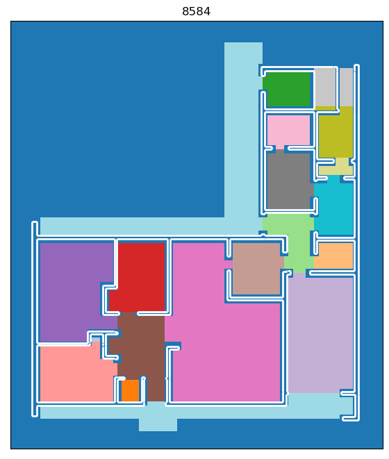
Practically speaking, a geometry is a dotdict with the following attributes:

id

An integer uniquely identifying this geometry

walls

An (M, 2, 2)-array of endpoints of the walls of the geometry, given as (x, y) coordinates in units of meters.

One ‘weird’ restriction is that all the coordinates should be strictly positive. This is not a fundamental restriction, it just makes a bunch of code elsewhere in megastep simpler if the geometry can be assumed to be in the top-right quadrant.

lights

An (N, 2)-array of the locations of the lights in the geometry, again given as (x, y) coordinates

As with the walls, the lights should all have strictly positive coordinates.

masks

An (H, W) masking array describing the rooms and free space in the geometry.

The mask is aligned with its lower-left corner on (0, 0), and each cell is res wide and high. You can map between the (i, j) indices of the mask and the (x, y) coords of the walls and lights with centers() and indices()

The mask is -1 in cells touching a wall, and otherwise 0 in free space or positive integer if the cell is in a room. Each room gets its own positive integer.

res

A float giving the resolution of masks in meters.

The geometry is a dotdict rather than a class because when writing your own environments, it’s common to want to nail extra bits of information onto the side of the default geometry. That could be handled by subclassing, but I have a personal aversion to inheritance hierarchies in research code.

Agents

‘Agents’ can - confusingly - refer to a few different things in megastep. Which is meant is usually clear from context.

For one, the agent is the thing that interacts with the environment. It receives observations and emits actions, and usually it’s controlled by a neural net of some sort. You’ll often see the Pytorch module that holds the policy network being called agent.

For two, there’s also the agent-as-a-specific-model-and-camera-in-the-world. Confusingly though, the agent-as-a-neural-net can have more than one agent-as-a-model-and-camera that it receives observations from and emits actions for. For example, a drone swarm might have a single net that controls multiple drones.

In terms of behaviour, agents-as-models-and-cameras are represented by the Agents datastructure. This datastructure holds the agents’ positions and velocities, and when you call render(), the models in the world are updated to match the positions in the datastructure. The positions in the datastructure are also the ones used for rendering.

Scenery

Scenery is the information the renderer uses to produce observations and the physics engine uses bounce agents off of things. It is usually - though not necessarily - created by feeding geometries into scenery(), and it’s represented by the Scenery object.

Versus Geometry

There are a couple of things that separate scenery from geometry. First, scenery has texture and light intensity information that the source geometry is missing. This separation is because generating randomly-varying textures and lights is a lot easier than generating high-quality random geometries.

Secondly, a geometry only represents a single environment, while scenery represents a multitude - typically thousands. The Scenery object stores all this information in a dense format that the rendering and physics kernels can access efficiently.

Finally, a geometry doesn’t specify how many agent-models there are. Scenery does.

Implementation Details

The most important - and most confusing - parts of the scenery object are the lines and the textures.

The lines are a ragged giving the, well, lines for each environment. If you index into it at position i, you’ll get back a (n_lines, 2, 2)-tensor giving the endpoints of all the lines in that environment. The first n_agents * model_size lines of each environment are the lines of that environment’s agents, with the first agent occupying the first model_size lines and so on.

The textures are another ragged giving the texels for each line. The texels are a fixed-resolution (5cm default) texture for the lines. If line j is 1m long, then indexing into the textures at j will give you a 20-element array with the colour of the line in each 5cm interval.

As well as the lines and textures, there’s also baked, which the bake() call fills with precomputed illumination.

Rendering

Rendering in megastep is extremely simple.

When the Scenery is first created, bake() is called to pre-compute the lighting for all wall texels. Wall texels are the colours and patterns that are applied to the walls. They make up the vast majority of the texels in the world, so this baking step saves a lot of runtime. The downside is it means that megastep does not have any dynamic shadows.

Then, each timestep render() gets called.

The first thing it does is update the positions of the agent-model’s lines to match the positions given in Agents.

Next, it computes dynamic lighting for the agent texels of the world. Agent texels are the colours and patterns that are applied to the agent-models. There aren’t many agent texels, so although this has to be done every timestep (unlike the wall’s baked lighting) it’s fast. The results of the dynamic lighting are used to update the baked tensor, because I am bad at naming things.

Then, each agent has a camera of a specified horizontal resolution and field of vision, and rays are cast from the camera through each pixel out into the world. These rays are compared against the scenery lines, and whichever line is closest to the camera along the ray is recorded. These ‘hits’ give the indices and locations tensors.

Finally, these line indices and locations are used to index into the textures tensor and lookup what the colour should be at that pixel. Linear interpolation is used when a hit falls between two texels, and after multiplying by the light intensity the result is returned in the screen tensor.

When you visualize the screen tensor yourself, make sure to gamma_encode() it, else the world will look suspiciously dark.

You can see the exact implementation in the render definition of the kernels file.

Physics

Physics in megastep is extremely simple.

Typically an environment will set the Agents velocity tensors at each timestep. Then when physics() is called, the agent’s position tensors are updated based on their velocities and any collisions that happen.

As far as collisions go, agents are modelled as discs slightly larger than their Models. When a disc looks like its current velocity will take it through a wall - or another disc - in the current timestep, the point is found where the collision would happen, and the the agent’s position is set to be a little short of that point.

As well as setting the position, when any sort of collision happens the velocity of the agent is set to zero. Not very physical, but simple!

The physics() call returns a Physics object that can tell you whether a collision occured.

You can see the exact implementation in the physics definition of the kernels file.

Plotting

megastep itself isn’t prescriptive about how environments are visualized, but here are some suggestions.

Implementing plotting megastep-style means implementing two methods.

First, there’s a state() method that returns one sub-environment’s current state as a dotdict of tensors. Then, there’s a plot_state() classmethod that takes a numpyify()’d version of that state and returns a matplotlib figure.

The various modules that are commonly used in constructing megastep environments often have their own state and plot_state methods, which can make implementing the methods for your library as simple as calling the module methods. See the the demo envs for examples.

The reason for separating things into get-state and plot-state is that frequently getting the state is much, much faster than actually plotting it. By separating the two, the get-state can be done in the main process, and the plot-state can be done in a pool of background processes. This makes recording videos of environments much faster, and there are tools like ParallelEncoder to help out with this.

The reason for getting torch state but passing numpy state is because the state method turns out to be useful for lots of other small tasks, and if it returned numpy state directly it’d get in the way of those other things. It’s also because initializing Pytorch in a process is pretty expensive and burns about a gigabyte of GPU memory per process. This can be lethal if you’ve got some memory-intensive training going on in the background.

The reason for making the plot-state method a classmethod is so that the function can be passed to another process without dragging the large, complex object it’s hanging off of with it.

Models

Models are the set of lines that are used to represent agents in the world. Right now there can only be one model that’s shared by all agents, though each agent’s texture can be different. The model is defined by the model tensor, and when you call render() the model is translated and rotated into the lines.

Right now there’s a bit of bad coding where the radius of the disc used for physics calculations and for the near clipping plane is hard-coded as AGENT_RADIUS. If you decide to alter the model, make sure to alter this too.

TODO: Derive the AGENT_RADIUS from the model as necessary

Subpackages

There are several roughly independent pieces of code in megastep.

Firstly there’s megastep itself. This is the environment development library, with its CUDA kernels and modules and raggeds.

Then there’s cubicasa, which is a database of 5000 floorplans. The cubicasa module while small in and of itself, requires some hefty geospatial dependencies. It uses these to cut the original floorplan SVGs into pieces and reassemble them as arrays that are useful for reinforcement learning research. It’s offered as an extra install because many users might want to avoid installing all those dependencies.

Finally there’s rebar. rebar is my - Andy Jones’s - personal reinforcement learning toolbox. While the bits of it that megastep depend on are stable and well-documented, the rest of it is not. That it’s still in the megastep repo is a bit of a historical artefact. One of my next tasks after getting megastep sorted is to get rebar equally well documented and tested, and then probably carve the unstable bits out into their own repo and package.

Decision & World

megastep isn’t prescriptive about how you hook your agent up to your environment, but here are some ideas that influence how the demo envs were written.

The demo envs’s step methods depart from the OpenAI Gym API in that they all take decision objects and return world objects.

decision objects are arrdicts with an actions key. The actions value should correspond to the environment’s action space. For example, suppose the environment has one sub-environment and this action space:

from megastep import spaces
from rebar import dotdict
action_space = dotdict.dotdict(
    movement=spaces.MultiDiscrete(2, 7),
    fire=spaces.MultiDiscrete(2, 2))

Then the corresponding decision object might be

from rebar import arrdict
decision = arrdict.arrdict(
    actions=arrdict.arrdict(
        movement=torch.as_tensor([[5, 6]]),
        fire=torch.as_tensor([[0, 1]])))

The advantage of passing the actions inside a dict is that you’ll often find you want return extra information from your agent (like logits), and this lets the environment decide which bits of the agent’s output it wants to use. The alternative is to return the actions and the other information separately, but then the experience collection loop would need to be aware of the details of the agent and environment.

Similarly, world objects are arrdicts with an obs key. The obs value should correspond to the environment’s observation space. As with decision, the advantage of this is that the environment can return much more than just obs, and the agent can pull out what it wants without the experience collection loop being any the wiser.

All together, the experience collection loop will typically look like this:

world = env.reset()
for _ in range(64):
    decision = agent(world)
    world = env.step(decision)

If you’re still confused, take a look at the minimal env tutorial or the demo envs.

Spaces & Heads

megastep isn’t prescriptive about how you hook your agent up to your environment, but here are some ideas that influence how the demo envs were written.

Often when you’re playing with environments, you’re not interested in the environment in isolation. Instead, you’re interested in how changing bits of the environment changes how agents train on that environment. Two of the most common ways to change the environment are changing the observations and changing the actions.

Something you’ll find frequently frustrating if you do this regularly is that every time you change the observations or actions, you have to change the architecture of your agent. Thing is, how you change the agent is pretty mechanical: when you change the observations, you change the input layers, and when you change the actions, you change the output layers.

As such, the demo envs declare their observations and actions using dicts of spaces. The spaces are little more than containers for the expected shape of the observations or actions. Most of their actual value comes from heads.

Intake heads like MultiImage take some sort of input described by an input space and output a vector of a fixed width. In particular, there is a ConcatIntake that concatenates the vectors of multiple other heads and outputs a vector of a fixed width. Together these mean you can offer up a dotdict of spaces as your observation space on your environment, and by writing your input layer in your agent as

intake = spaces.intake(env.observation_space)

you get a intake module that will take observations from the environment - whatever those observations turn out to be - and outputs a vector of fixed width that’s suitable for passing into some fully-connected or LSTM or transformer core.

Output heads like MultiDiscrete do the converse: they take a vector of a fixed width and output something that conforms to what the action space describes. Again, there’s a DictOutput that takes a vector of fixed width and outputs a vector of fixed width for each subsidiary action space. Writing your output layer as

output = spaces.output(env.action_space)

you get a output module that will take a vector from your fully-connected/LSTM/transformer core and outputs things suitable for your environment to consume.

Exactly how you convert spaces into network layers is up to you. The setup in heads suggests one layout, but it’s entirely personal taste.

Env Patterns

TODO-DOCS Env patterns concept

• Use modules where possible

• Get your plotter working first

• A display method

• A _reset method

• A _observe method

• n_envs and device